At the moment there is a wonderful course running at Standford University, called CS231n - Convolutional Neural Networks for Visual Recognition, held by Andrej Karpathy, Justin Johnson and Fei-Fei Li. Fortunately all the course material is provided for free and all the lectures are recorded and uploaded on Youtube. This class gives a wonderful intro to machine learning/deep learning coming along with programming assignments.

Batch Normalization

One Topic, which kept me quite busy for some time was the implementation of Batch Normalization, especially the backward pass. Batch Normalization is a technique to provide any layer in a Neural Network with inputs that are zero mean/unit variance - and this is basically what they like! But BatchNorm consists of one more step which makes this algorithm really powerful. Let’s take a look at the BatchNorm Algorithm:

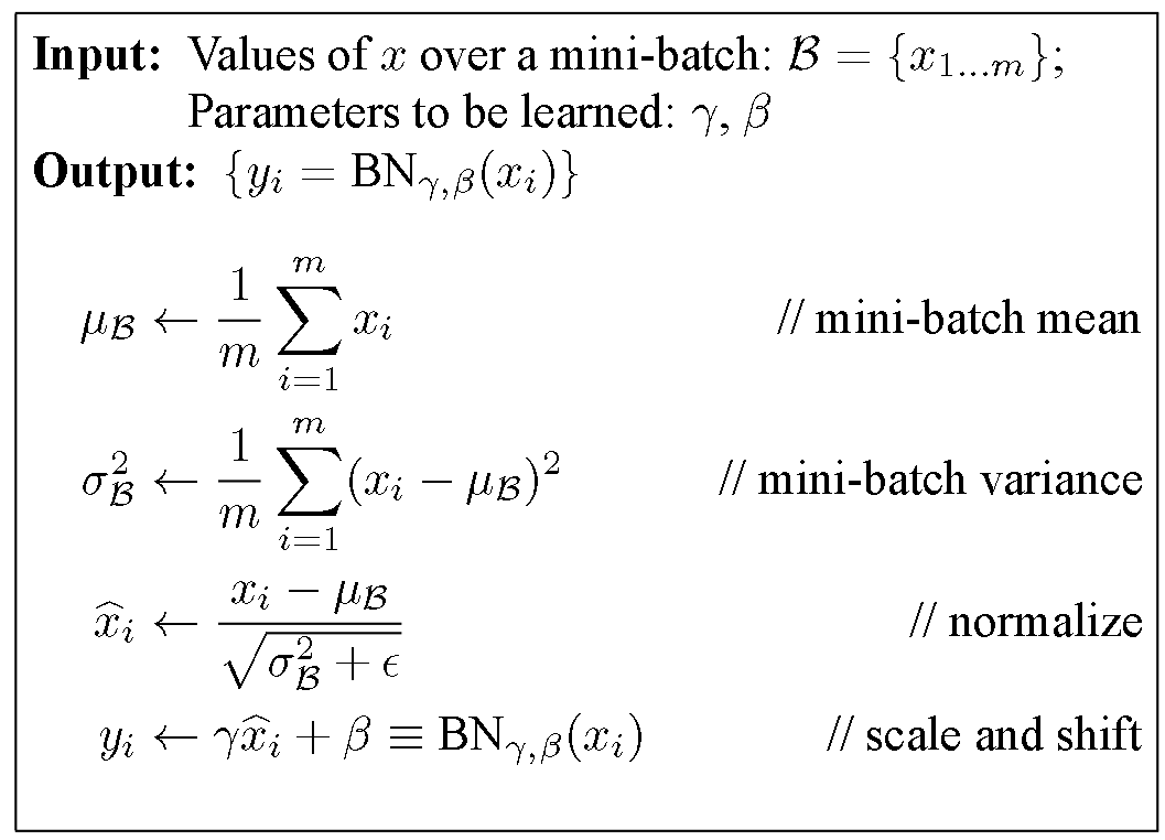
Algorithm of Batch Normalization copied from the Paper by Ioffe and Szegedy mentioned above.

Look at the last line of the algorithm. After normalizing the input x the result is squashed through a linear function with parameters gamma and beta. These are learnable parameters of the BatchNorm Layer and make it basically possible to say “Hey!! I don’t want zero mean/unit variance input, give me back the raw input - it’s better for me.” If gamma = sqrt(var(x)) and beta = mean(x), the original activation is restored. This is, what makes BatchNorm really powerful. We initialize the BatchNorm Parameters to transform the input to zero mean/unit variance distributions but during training they can learn that any other distribution might be better. Anyway, I don’t want to spend to much time on explaining Batch Normalization. If you want to learn more about it, the paper is very well written and here Andrej is explaining BatchNorm in class.

Btw: it’s called “Batch” Normalization because we perform this transformation and calculate the statistics only for a subpart (a batch) of the entire trainingsset.

Backpropagation

In this blog post I don’t want to give a lecture in Backpropagation and Stochastic Gradient Descent (SGD). For now I will assume that whoever will read this post, has some basic understanding of these principles. For the rest, let me quote Wiki:

Backpropagation, an abbreviation for “backward propagation of errors”, is a common method of training artificial neural networks used in conjunction with an optimization method such as gradient descent. The method calculates the gradient of a loss function with respect to all the weights in the network. The gradient is fed to the optimization method which in turn uses it to update the weights, in an attempt to minimize the loss function.

Uff, sounds tough, eh? I will maybe write another post about this topic but for now I want to focus on the concrete example of the backwardpass through the BatchNorm-Layer.

Computational Graph of Batch Normalization Layer

I think one of the things I learned from the cs231n class that helped me most understanding backpropagation was the explanation through computational graphs. These Graphs are a good way to visualize the computational flow of fairly complex functions by small, piecewise differentiable subfunctions. For the BatchNorm-Layer it would look something like this:

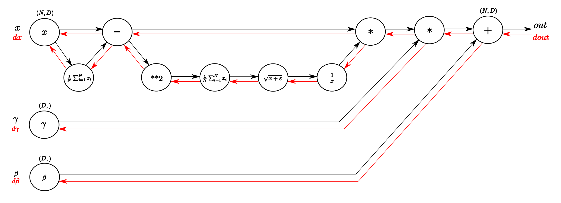
Computational graph of the BatchNorm-Layer. From left to right, following the black arrows flows the forward pass. The inputs are a matrix X and gamma and beta as vectors. From right to left, following the red arrows flows the backward pass which distributes the gradient from above layer to gamma and beta and all the way back to the input.

I think for all, who followed the course or who know the technique the forwardpass (black arrows) is easy and straightforward to read. From input x we calculate the mean of every dimension in the feature space and then subtract this vector of mean values from every training example. With this done, following the lower branch, we calculate the per-dimension variance and with that the entire denominator of the normalization equation. Next we invert it and multiply it with difference of inputs and means and we have x_normalized. The last two blobs on the right perform the squashing by multiplying with the input gamma and finally adding beta. Et voilà, we have our Batch-Normalized output.

A vanilla implementation of the forwardpass might look like this:

def batchnorm_forward(x, gamma, beta, eps):

  N, D = x.shape

  #step1: calculate mean
  mu = 1./N * np.sum(x, axis = 0)

  #step2: subtract mean vector of every trainings example
  xmu = x - mu

  #step3: following the lower branch - calculation denominator
  sq = xmu ** 2

  #step4: calculate variance
  var = 1./N * np.sum(sq, axis = 0)

  #step5: add eps for numerical stability, then sqrt
  sqrtvar = np.sqrt(var + eps)

  #step6: invert sqrtwar
  ivar = 1./sqrtvar

  #step7: execute normalization
  xhat = xmu * ivar

  #step8: Nor the two transformation steps
  gammax = gamma * xhat

  #step9
  out = gammax + beta

  #store intermediate
  cache = (xhat,gamma,xmu,ivar,sqrtvar,var,eps)

  return out, cache

Note that for the exercise of the cs231n class we had to do a little more (calculate running mean and variance as well as implement different forward pass for trainings mode and test mode) but for the explanation of the backwardpass this piece of code will work. In the cache variable we store some stuff that we need for the computing of the backwardpass, as you will see now!

The power of Chain Rule for backpropagation

For all who kept on reading until now (congratulations!!), we are close to arrive at the backward pass of the BatchNorm-Layer. To fully understand the channeling of the gradient backwards through the BatchNorm-Layer you should have some basic understanding of what the Chain rule is. As a little refresh follows one figure that exemplifies the use of chain rule for the backward pass in computational graphs.

The forwardpass on the left in calculates `z` as a function `f(x,y)` using the input variables `x` and `y` (This could literally be any function, examples are shown in the BatchNorm-Graph above). The right side of the figures shows the backwardpass. Receiving `dL/dz`, the gradient of the loss function with respect to `z` from above, the gradients of `x` and `y` on the loss function can be calculate by applying the chain rule, as shown in the figure.

So again, we only have to multiply the local gradient of the function with the gradient of above to channel the gradient backwards. Some derivatives of some basic functions are listed in the course material. If you understand that, and with some more basic knowledge in calculus, what will follow is a piece of cake!

Finally: The Backpass of the Batch Normalization

In the comments of aboves code snippet I already numbered the computational steps by consecutive numbers. The Backpropagation follows these steps in reverse order, as we are literally backpassing through the computational graph. We will know take a more detailed look at every single computation of the backwardpass and by that deriving step by step a naive algorithm for the backward pass.

Step 9

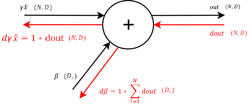
Backwardpass through the last summation gate of the BatchNorm-Layer. Enclosed in brackets I put the dimensions of Input/Output

Recall that the derivative of a function f = x + y with respect to any of these two variables is 1. This means to channel a gradient through a summation gate, we only need to multiply by 1. For our final loss evaluation, we sum the gradient of all samples in the batch. Through this operation, we also get a vector of gradients with the correct shape for beta. So after the first step of backpropagation we already got the gradient for one learnable parameter: beta

Step 8

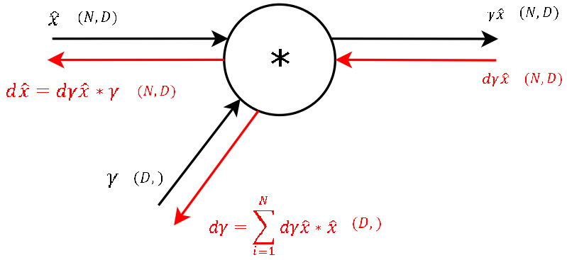
Next follows the backward pass through the multiplication gate of the normalized input and the vector of gamma.

For any function f = x * y the derivative with respect to one of the inputs is simply just the other input variable. This also means, that for this step of the backward pass we need the variables used in the forward pass of this gate (luckily stored in the cache of aboves function). So again we get the gradients of the two inputs of these gates by applying chain rule ( = multiplying the local gradient with the gradient from above). For gamma, as for beta in step 9, we need to sum up the gradients over dimension N. So we now have the gradient for the second learnable parameter of the BatchNorm-Layer gamma and “only” need to backprop the gradient to the input x, so that we then can backpropagate the gradient to any layer further downwards.

Step 7

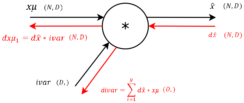
This step during the forward pass was the final step of the normalization combining the two branches (nominator and denominator) of the computational graph. During the backward pass we will calculate the gradients that will flow separately through these two branches backwards.

It’s basically the exact same operation, so lets not waste much time and continue. The two needed variables xmu and ivar for this step are also stored cache variable we pass to the backprop function. (And again: This is one of the main advantages of computational graphs. Splitting complex functions into a handful of simple basic operations. And like this you have a lot of repetitions!)

Step 6

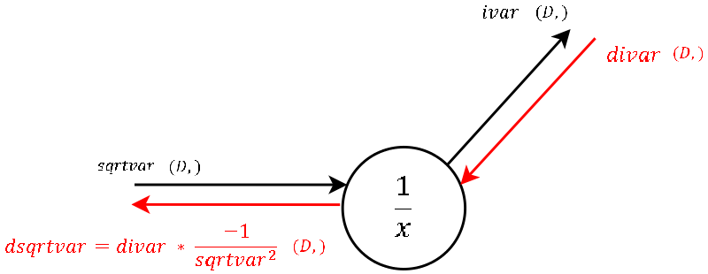
This is a "one input-one output" node where, during the forward pass, we inverted the input (square root of the variance).

The local gradient is visualized in the image and should not be hard to derive by hand. Multiplied by the gradient from above is what we channel to the next step. sqrtvar is also one of the variables passed in cache.

Step 5

Again "one input-one output". This node calculates during the forward pass the denominator of the normalization.

The calculation of the derivative of the local gradient is little magic and should need no explanation. var and eps are also passed in the cache. No more words to lose!

Step 4

Also a "one input-one output" node. During the forward pass the output of this node is the variance of each feature `d for d in [1...D]`.

The calculation of the derivative of this steps local gradient might look unclear at the very first glance. But it’s not that hard at the end. Let’s recall that a normal summation gate (see step 9) during the backward pass only transfers the gradient unchanged and evenly to the inputs. With that in mind, it should not be that hard to conclude, that a column-wise summation during the forward pass, during the backward pass means that we evenly distribute the gradient over all rows for each column. And not much more is done here. We create a matrix of ones with the same shape as the input sq of the forward pass, divide it element-wise by the number of rows (thats the local gradient) and multiply it by the gradient from above.

Step 3

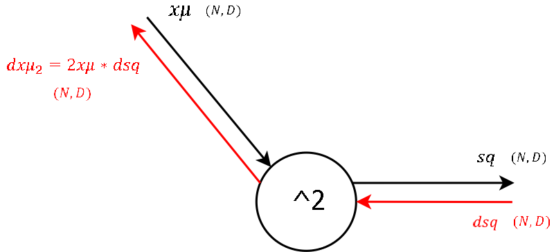
This node outputs the square of its input, which during the forward pass was a matrix containing the input `x` subtracted by the per-feature `mean`.

I think for all who followed until here, there is not much to explain regarding the derivative of the local gradient.

Step 2

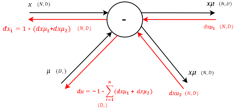
Now this looks like a more fun gate! two inputs-two outputs! This node subtracts the per-feature mean row-wise of each trainings example `n for n in [1...N]` during the forward pass.

Okay lets see. One of the definitions of backprogatation and computational graphs is, that whenever we have two gradients coming to one node, we simply add them up. Knowing this, the rest is little magic as the local gradient for a subtraction is as hard to derive as for a summation. Note that for mu we have to sum up the gradients over the dimension N (as we did before for gamma and beta).

Step 1

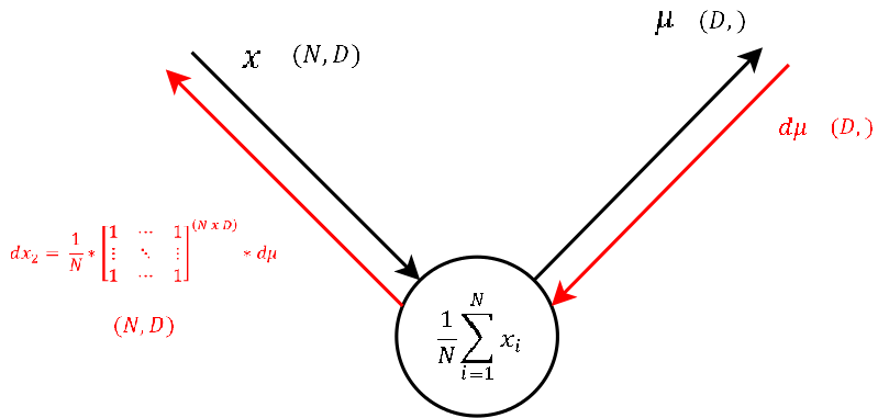
The function of this node is exactly the same as of step 4. Only that during the forward pass the input was `x` - the input to the BatchNorm-Layer and the output here is `mu`, a vector that contains the mean of each feature.

As this node executes the exact same operation as the one explained in step 4, also the backpropagation of the gradient looks the same. So let’s continue to the last step.

Step 0 - Arriving at the Input

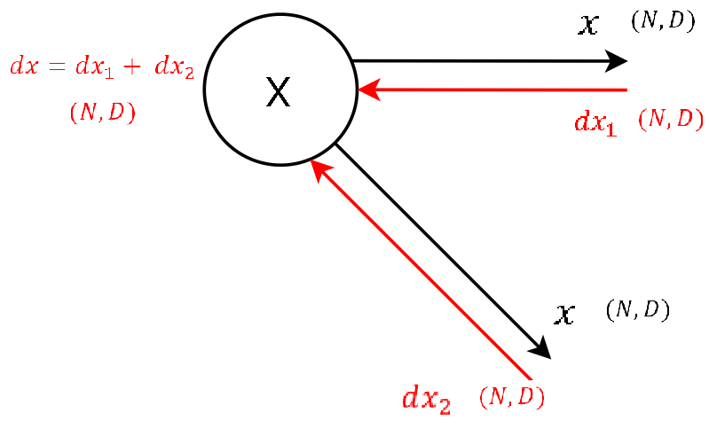
I only added this image to again visualize that at the very end we need to sum up the gradients dx1 and dx2 to get the final gradient dx. This matrix contains the gradient of the loss function with respect to the input of the BatchNorm-Layer. This gradient dx is also what we give as input to the backwardpass of the next layer, as for this layer we receive dout from the layer above.

Naive implemantation of the backward pass through the BatchNorm-Layer

Putting together every single step the naive implementation of the backwardpass might look something like this:

def batchnorm_backward(dout, cache):

  #unfold the variables stored in cache
  xhat,gamma,xmu,ivar,sqrtvar,var,eps = cache

  #get the dimensions of the input/output
  N,D = dout.shape

  #step9
  dbeta = np.sum(dout, axis=0)
  dgammax = dout #not necessary, but more understandable

  #step8
  dgamma = np.sum(dgammax*xhat, axis=0)
  dxhat = dgammax * gamma

  #step7
  divar = np.sum(dxhat*xmu, axis=0)
  dxmu1 = dxhat * ivar

  #step6
  dsqrtvar = -1. /(sqrtvar**2) * divar

  #step5
  dvar = 0.5 * 1. /np.sqrt(var+eps) * dsqrtvar

  #step4
  dsq = 1. /N * np.ones((N,D)) * dvar

  #step3
  dxmu2 = 2 * xmu * dsq

  #step2
  dx1 = (dxmu1 + dxmu2)
  dmu = -1 * np.sum(dxmu1+dxmu2, axis=0)

  #step1
  dx2 = 1. /N * np.ones((N,D)) * dmu

  #step0
  dx = dx1 + dx2

  return dx, dgamma, dbeta

Note: This is the naive implementation of the backward pass. There exists an alternative implementation, which is even a bit faster, but I personally found the naive implementation way better for the purpose of understanding backpropagation through the BatchNorm-Layer. This well written blog post gives a more detailed derivation of the alternative (faster) implementation. However, there is a much more calculus involved. But once you have understood the naive implementation, it might not be to hard to follow.

Some final words

First of all I would like to thank the team of the cs231n class, that gratefully make all the material freely available. This gives people like me the possibility to take part in high class courses and learn a lot about deep learning in self-study. (Secondly it made me motivated to write my first blog post!)

And as we have already passed the deadline for the second assignment, I might upload my code during the next days on github.